
The executing proces of this program is divided of six independent algorisms, that are used to predict the best companies to invest in. All the process is repeated for the 2247 companies every weekday while in the weekend it makes a weekly report to check how are the predictions going. The daily execution takes 22:30 hours and its executed in my personal server in local.
Next I will explain the 6 algorithms in detail:
Technical analisis:
For the technical analysis, I created a ML model that predict the price of the stock market using the Logistic Regression algorithm. This model study the evolution of the stock price of a company (technical analysis) and try to predict it using the deviation of the stock price of different periods of time.Technical analysis is based in the stock price of the companies, and for this reason, the price of the stock is going to be our main raw data. The data used in this algorithm come from the first of 2012 to the last day, due to the data fited in the model is actualized every day.
This ML algorism is fited with 18 total variables (17 independent variables + 1 dependent variable), separated into 4 different groups: 1) Variables Balance, 2) Comparative with NASDAQ, 3) Distance from maximum and minimum and 4) Target variable (dependent variable). All the 18 variables are calculated for each row of data, or what is the same for each day of the stock data. Once we have created all the variables, we will be able to find trends and analyse the values of variables that perform better and have a better return on the inversion.
1) Variables Balance:
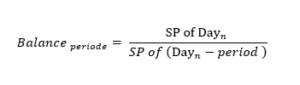
This group contains 7 different variables, and the objective of this group is to fit the stock chart of the company in our model. To convert a graph into a numerical value, we create the balances or desviation which is the evolution of the company during a period of time. For this model we had created the balances of the following different periods of time: 3 years, 1.5 years, 7 months, 3 months, 3 weeks, 1 week, and 2 days. With the seven variables, we are going to be able to recreate the evolution of the stock of the last 3 years, with a numeric recreation equivalent to the stock chart.
The equation for Balance variables:
SP = Stock Price
Day = Day or row with daily data that contain the SP
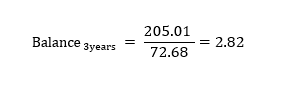
SP= Price stock MSFT 31/07/2020 = 205.01
(Dayn – period) = (31/07/2020 – 3 years) = 31/07/2017
Price stock MSFT 31/07/2017= 72.68
2) Variables comparative with NASDAQ:
These variables are based in the same system as the Variables Balance, but instead of creating the balance for the company, is going to do it for the NASDAQ Index. There are 3 different periods of time for these variables: 1.5 years, 3 months and one week. When the 3 NASDAQ balances are created, we are going to save the variables and create 3 extra variables. To create the other 3 variables, we are going to compare the results of the NASDAQ balances with the balances of the companies for the same periods, and return 1 if the balance of NASDAQ is lower than the one of the company or 0 if is higher. Therefore, if the company is growing more than NASDAQ, it will return 1, and 0 if not. This group of variables will help us understand how the company is behaving compared to the NASDAQ Index, and how the market performing.
3) Variable distance from maxim and minim:
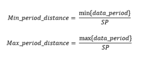
The variable distance from maxim and minim are going to analyse how is stock price respect a local maxim or minim. As the other variables in this there are also different periods of time, in this case there are only two different periods 1 month and 4 months. To Analyse the distance from the minim and the maximum, it is necessary to obtain the data of the last month or the last 4 months, depend of the period. Then we find the max and the minim of the stock price of that period. Once you have the minim or the maxim you must divide the actual value of the stock price for the mini mor maxim of that period. As a result, we are going to know how much the variable fluctuated in that period, and the actual state of the stock price.
The equation of distance variable:
SP = Stock Price
data_ period = Daily data of the SP during all the periods.
4) Target variable:
The target variable or dependent variable is what are going to use to predict our algorism. In our case, this is going to be the return of the investment of a specific period of time. Since we have a table with all the historic stock prices, we can find out the future price of a past date. The method is similar as the balance variable but instead of getting the past data we use the “future” data of that specific past date. Using this methodology, I can know the return of the inversion, of a determinate period.
The equation for the Target variable:
SP = Stock Price
Day = Day or row with daily data that contains the SP
Period = The amount of time of the variable

Once all the 18 variables are created, the next step is to prepare the data by grouping it and train the data with the logistic regression algorism in order to make the prediction.
Group the data:
One of the most used technics for obtaining high-value variables for a ML model is to create groups for the different features or variables. This helps the ML algoristhm find trends in the data, and is also easier for data visualization. With this method, we group the variables according to their behaviour on a characteristic that we want to study. In our case, the behaviour we want to study is the correlation of the variables with the target variable in the different groups. Also, it is important that the groups have a similar distribution of data, as if one group has a small sample of the data, the results might not be accurate.
In order to create the groups, it is important to check the distribution of data on the groups to see the behaviour of the groups in our target variable. In our case, once we group the variables, we can see what the average return of the inversion for each group is, and also the average time when the return of the inversion is negative. It is recommended to keep creating groups until we find the parameters that maximize the trend of the performance of the target variable.
Apply the Logistic Regression:
The ML modelling starts by defining the target variable and the features. The features are going to be all 17 variables which have been grouped, and the target variable if the return was higher or lower than the limit determined according to the period on the Target Variable section. We are going to save the target variable on a pandas series, and the features on a bidimensional array. Next, we going to split the data in training and testing, by defining the percentage of data that we are going to train and test. In our case, we are going to train the 80% of the data and test the 20%. This means that we going to take an aleatory sample of 80% of the data to fit into the Logistic Regression algorithms in order to study the data and find an accurate function. Once we enter the target variable, the features and we defined the percentage of train, the sklearn library will get the training features and training target variable and fit them into a function where we will apply the Logistic Regression algorism. That function is going to return to us a logistic regression function of our training data that we are going to use for the predictions. Finally, we are going to apply the function to our testing data and see how the model predicts the non-trained data, or data that the model never saw. We are going to use the accuracy score and more ratios that we are going to see next, to prove the performance of our model. Finally once the expected accuracy is optined it’s time to apply the trained algorithm to the daily data to obtain the result of the prediction.
RM method:
The RM method is an algorithm I create to avoid the lax of standardization of the data and the poor impact of the most valued variable. The algorithm is based in the evaluation of financial variables according to their return, and the relative return over all the different variables. To evaluate the variables, the algorithm is going to return a value between -1 and 2, where -1 will be assigned to the variable with worse performance and 2 to the best. Once we evaluate all the variables, we are going to add the values of the different variables and we will obtain the final value that will estimate how good is the company according to the variables estudies. As we can expect as closer to 2 the final value the better it should perform the company.
The RM algo is a applied in 2 of the 6 independent algorisms with different data sets, however the process is exactly the same. Next we are going to explain the benefits of this algorithm, the data and then the process.
Benefits:
The main benefit of the RM algorithm is that works well with unstadirsed data. As the model runs 2247 companies with different data and with different missing values executing a ML algorism with that amount of missing data could cause unexpected results that would impact the performance of the program. Due to the RM algorithm manage well the missing values, making them have a non-impact in the results, makes the algorithm works well with this data sets.
Another positive point of the RM algo is to consider the impact of the worse variables and reward the variables that perform better. During the study of the RM algorism I wanted to remark the importance of the variables that had a bad performance, because is the once I want to avoid, and also give and extra positive point to the best performance variables because are the one I want more. The variables that are at the extremes (-1 and 2) are the once that would impact more and the most relevant once. The evaluation of the companies goes from -1 to the worse and 2 the best, however, there is the same amount of values between (-1, 0) and (0 , 2), this is because I wanted to remark more the best performance variables, due to I am more interested in remark the variables that will maximize the ROE than penalize the once that perform worse. This means that most values will have a value around 0, and so their performance doesn’t have a considerable impact in the return, and so in the RM algorism.
During the study or creation of this algorithm I tried different limit values to select the best one. Next, I’m going to explain the different values I tried and why I discard:
– [-1, 1] With this limit range I obtain a distribution where almost all the values where in the middle, making the most valuable variables don’t have same impact as the final values selected. So the better performance variables that is what will make our prediction work better is more likely to have less impact.
– [-2,-1] ^3 – [1, 2]^3: In this case I used the cube exponential, to be able to do exponential at negative values. The middle values doesn’t affect at the final value because the extremes have a huge impact due the exponential.
Finally, our algorithm is pretty good giving the right value to each variable. As we will see in the process, the RM algorithm consider all the variables to define the value of each variable. This makes that the algorithms don’t underestimate a variable and that the variables have the right impact in the final value. With this even if a variable hasn’t a good performance it doesn’t underestimate it and it give the exact mathematical / theoretical number that should be applied in the result.
Data:
This algorithm works with labled data so can be considered as a supervised learning. As I said this algorithm is applied in two different independent parts: the financial statements 1 with 28 financial metrics (*1) and the second, Financial growth, which is trained with 38 variables (*2). Both algorisms are trained with data from 1990 to first of 2022. In total there are more than 300k rows of historic data.
The variables we are going to use are financial variables or metrics obtained from each quarterly financial report, these variables are processed to obtain the deviation between reports or between quarters. So instead of having a database with values of the cost of revenue or net income, we are going to have the quarterly deviation of that variable in percentage. Working with the percentage of deviation is going to allow me to use data from different companies, and then study how the deviation in each variable affects the investment return.
Training:
The first step in the training process is to define the variables to study in the RM method. It’s important that all the variables selected has the same format, in our case percentage. Once defined all the variables, the algorism will group each variable in four groups, according to the performance of the variable. The groups will be the next: the variables with the 25% higher performance, the variables with the 25% lowest performance, the variables with average performance (between 25% higher- 25% lower) and the missing or null values. So if for example, the average net income deviation is 1.03% and there is a company with that net income deviation, will be grouped in the group with average performance (between 25%highier- 25%lower), and so if the top 25% higher net income deviation starts at 6% any variable above 6% deviation will be at group 25% higher.
The next step in the process is to discard the variables with non-impact or no relevance, in order to dismiss underrepresented groups that have less than 5% of representation over all the data set. These groups will be considered as a non-relevant variables or null due to there isn’t enough data to work with. With the rest of the variables, the program will calculate the average return for all the groups and add the result in a dictionary with “VarName_GroupName” as a key and the average return as a value.
Next, the RM algorithm will apply the Range Method to all the variables. The first step in this method is to define the limits and the middle values. The group of variables with the minimum average return of the dictionary will take the value -1, and the max return will take the value 2 and the average will be 0. Once defined all the limits the next point will be to define all the groups between -1 and 2 according to their return. So the variables that perform worse than average will have a negative value and the once better than average will have a positive value between 0 and 2. The null values and the values with less than 5% representation will automatically have the value 0 assigned so doesn’t affect to the algorism performance. This process is calculated by the next equation:
if value > mean_v0:if value <= mean_v0:y = max_ - mean_v0y = value - min_x = value - mean_v0x = mean_v0 - min_technic_value = round(((x / y) * 2), 4)technic_value = round((( y / x ) - 1), 4)
With this equation, all the variables will have the exact value according to their risk o they rentability. The result is going to be added in a dictionary in order to create a function for each variable. The functions will do all the process in the simplest way. Due to I already create the groups and assigned the value to each variable, the function will only create the four groups and return the value assigned in the range method, so the process will be fast and not powering consuming. Once all the functions are created for all the variables, apply this algo will be as easy as apply all the functions to the daily data and add all the results to obtain the final value. This final value is going to be a technical estimation of how likely the company will maximize the return according to the historical data, being values close to two the most likely and -1 the less likely.
Financial statements 1 (*1): Revenue, cost of revenue, gross profit, gross profit ratio, research and development expenses, general and administrative expenses, selling and marketing expenses, selling general and administrative expenses, other expenses, operating expenses, cost and expenses, interest income, interest expense, depreciation and amortization, EBITDA ratio, operating income, operating income ratio, total other income expenses net, income before tax, income before tax ratio, income tax expense, net income, net income ratio, eps, eps diluted, weighted average shs out, weighted average shs out dil.
Financial growth (*2): Growth cash and cash equivalent, growth short-term investments, growth cash and short-term investments, growth net receivables, growth inventory , growth other current assets, growth total current assets, growth property plant equipment net, growth goodwill, growth intangible assets, growth goodwill and intangible assets, growth long term investments, growth tax assets, growth other non-current assets, growth total non-current assets, growth other assets, growth total assets, growth account payables, growth short term debt, growth tax payables, growth deferred revenue, growth other current liabilities, growth total current liabilities, growth long term debt, growth deferred revenue non-current, growth deferred tax liabilities non-current, growth other non-current liabilities, growth total non-current liabilities, growth other liabilities, growth total liabilities, growth common stock, growth retained earnings, growth accumulated other comprehensive income loss, growth other total stockholders equity, growth total stockholders equity, growth total liabilities and stockholders equity, growth total investments, growth total debt, growth net debt.
Financial ratios:
The use of financial ratios is one of the most extended technics of the fundamental analysis. Studying and examining the financial ratios allow the investors to understand the financial situation of a company. There are many financial ratios, and each one study an aspect of a business, for example the Cash Ratio determine the cash liquidity in the short term. The results of the financial ratios can be interpreted according to the maturity of a company, the industry or even the market situation. Therefore, even if two companies have similar results in the same ratio, this does not mean that they are in a similar situation. However, after a deep analisi of the results I found that there are some ranges in the ratios that maximize the return. We are going to use these ranges to score the different ratios with values 0, 1 and 2. Once all the ratios are evaluated the program will try to qualify and determine the general financial situation of the companies. The higher the result, the better the performance of the ratios. Finally, we are going to group the different ratios according to these four categories: 1. Stock price, 2 Liquidity, 3. Profitability and return and 4. Leverage.
– Stock price: The stock price group is going to analyse if the stock is overpriced or not by using the following two ratios: Price-to-earnings and Price/Earnings-to-Growth. These two ratios determine approximately if a stock is overpriced, or if it is going to be overpriced in future.
– Liquidity: Liquidity ratios measure a company’s ability to pay debt obligations and its margin of safety through the calculation of metrics, including the current ratio, quick ratio, and cash ratio.
– Profitability and return: Profitability ratios are a class of financial metrics that are used to assess a business’ ability to generate earnings relative to its revenue, operating costs, balance sheet assets, or shareholders’ equity over time. Meanwhile, the Return ratios offer several different ways to examine how well a company generates a return for its shareholders. Ratios used: Return On Assets (ROA), Return On Equity (ROE), Return On Capital Employed (ROCE), Gross Profit Margin, Net Profit Margin, Effective Tax Rate
– Leverage: A leverage ratio is any kind of financial ratio that indicates the level of debt incurred by a business entity against several other accounts on its balance sheet, income statement, or cash flow statement. These ratios provide an indication of how the company’s assets and business operations are financed (using debt or equity). Ratios used: Debt Ratio, Debt Equity Ratio, Long Term Debt To Capitalization, Total Debt To Capitalization, Interest Coverage, Cash Flow To Debt Ratio, Company Equity Multiplier
Evaluating the companies:
After defining the scores for all of the ratios, we are going to create a function for each group of ratios, so there are going to be 4 functions. Each function is going to contain the extraction of the respective ratios and the qualification of the ratios. The input of the function is going to be the ratios , meanwhile the output is going to be the average score of the ratios that the group contains. That result is going to give us an approximate image of the financial statement which the ratio measures. For example, if the output of the liquidity function is 1.66 ([ 2 Current Ratio + 2 Quick Ratio + 1 Cash Ratio] / 3 = 1.66), we are going to know that the company does not have any liquidity issues.
Finally, once we have the average of the groups, we are going to add them to obtain “the final result” value. The “final result” is going to give us an approximate image of the financial situation of the company. This result is going to be a value between zero and eight, and the higher the value, the better the financial situation of the company is. Using “the final result”, we are going to decide if the company we are analyzing is a good recommendation or not.
The fundamental analysis method gives our program a higher level of credibility. This is because it is giving our program the capacity to analyse and study the financial situation of the company using trusted and proved methods such as the study of the financial ratios. With this part, we use metrics and methods used by experts to simulate their decision making.
News:
The last variable is the news. As the news are a basic and essential font of information for any investor, I believed it was important to implement it in some way in the program. The point of implementing the news in the program is to consider the “real word” in the code, due to the fundamental data and the stock price doesn’t consider anything outside the company and the financial information. Implementing the news, makes the code able to consider important aspects such as how the company behaves and how the media or the public see the company. Also, the news can discover and consider an unforeseen event, that could detect a good opportunity to invest in or event prevent a highly risk investment.
To make the program detect the good and the bad news I made the program to read the news and “understand” them. To do that I created a code that studied 200.000 news. To extract the information or detect which new could be considered as positive I assign each new with its return on investment (the variation of the stock value between the day of the new was realised and 3 months later) then I split all the words of each news obtaining a total of 4.5 million words. Each word has assigned the return of their respective news, and because I obtained a 4.5 millions words there is many words that are repeated in multiple news. Doing the average return of each word we can see the impact that have the word and so detect the correlation of that new appearing on the new and the future return. Considering and analyzing all the different words that appears in a new and their average return, it’s possible to have an estimation of the expected return of any new.
To maximize the results of the program is important to consider the most relevant words and discard words that doesn’t apply may information to prevent overfitting of non-relevant words. To solve this problem I decided to discard the words like: to, have, the… that don’t apply any important information to news and so only consider the words that would contribute with more information.
The process of applying this algorism is simple, I obtain all the news of a company in the last month, because if it’s older probably the new is outdated, with a maxim limit of 100 news. The next step is to split all the words of the new and obtain the average return of each word from the table with the 4.5M words. Once we obtain all the averages return of the relevance words, we are going to do the average of the averages to obtain the expected return according to the news. This expected return is going to be the final output of the algorims.
Decision making process:
The final step of the program is to detect which company could be a good opportunity to invest in according to the results of the six independent algorism. To select the companies I created a method called “4 conditions”. This method is divided into 3 different steps: 1) The selection by results, 2) The discard by repetition and 3) The last check:
1) The selection by results is based in defining a binary variable for all the different results of all the six algorithms according to the value that will maximize the return. To determine which values are going to be a 1 or 0 I created a code that detects the best values of each algorism, based in the historic obtained during the testing. This process of selection is completely automatic, and it adjusts the parameters every month to maximize the results and adapt to a new circumstance. To define the limit, the code uses the historical data of the results (more than 150k), where there is the daily result of all the six algorism and the retutn. With these data sets the code will define the value that maximizes the result by using a Brute Force algorithm. The goal of that algorithm is to detect which values of each algorism has a better performance by defining a limit. I wanted to select a relatively big amount of companies due to it’s important to select the companies that are good at different algorithms, for this reason the code select at less the 15 % of the companies in each algorism. For this reason, the limit value will be between the 15% higher values and below and the 15% lower, then the code will get all the values between and is going to calculate the average return of the group above that value and the average return of the group below and save the values and the averages. Once the code calculates all the average, more than 100k and increases every month, will select the value with the higher average return, this value is going to be the limit. This process is repeated for all the 6 algorithm results getting the limit values that will define if the result of the algorism can be considered good or not. Once all the results are defined the code will add all the results of all the six algorims and the companies that obtain 4 or more good results are selected as a good possibility. Usually around 1,5% of the companies are selected or around 30 companies.
2) The next part is discarding the companies that pass the 4 conditions, but they are constantly repeated in the 4 conditions. During the analysis of this method, I saw that there is a considerable amount of companies that most day pass the 4 conditions, those companies have a considerable correlation with a lower return. For this reason I analyze which companies could be interesting to discard and which to once select. The analysis ends up by discard the companies that are repeated more than 15 times in the last month and discard the companies that is the first time that pass the 4 conditions. With this second step in the decision-making, the code makes sure that the companies selected are in the right moment to invest in not because the results are casually good.
3) The last step in the final decision is the last check. This final step is also divided in 3 checks: the amount of data, the performance and the news. In the amount of data check, the code will discard the companies that had been selected but the amount of missing data is enough to discard the company. The performance is going to analyze how the company selected has perform since the program has predicted the company until the moment of the final decision. The code will divide the stock price at the moment of prediction and the price once is doing the final decision, if the price has gone down the code will discard the company else it passes the check. The final check is the news, where the companies that have the variable news as good even if they have a large amoun amount of nulls or the price has gone down, the company is selected as a good opportunity to invest in.
The companies that pass all these 3 cheeks are the final output of the program or the companies I’m going to invest in. Usually, the amount companies that pass all the cheeks are between four and ten or the 0,25% of the total companies.
I have the program integrated with the interactive brokers API. This platform allows you to buy and sell stocks using python commands. Thanks to this API I’m able to invest in the most rational or non-emotional way due to the code is completely automatic and dose everything for me. To manage the investments with limited capital I created a code that will invest an X amount of money until no more is available. Also, to select the companies if there are multiple companies the program will diversify by regions and sectors, selecting the once that had obtain a better results in the last month.